Multigrid solvers
pyro solves elliptic problems (like Laplace’s equation or Poisson’s equation) through multigrid. This accelerates the convergence of simple relaxation by moving the solution down and up through a series of grids. Chapter 9 of the pdf notes gives an introduction to solving elliptic equations, including multigrid.
There are three solvers:
The core solver, provided in the class
MG.CellCenterMG2dsolves constant-coefficient Helmholtz problems of the form \((\alpha - \beta \nabla^2) \phi = f\)The class
variable_coeff_MG.VarCoeffCCMG2dsolves variable coefficient Poisson problems of the form \(\nabla \cdot (\eta \nabla \phi ) = f\). This class inherits the core functionality fromMG.CellCenterMG2d.The class
general_MG.GeneralMG2dsolves a general elliptic equation of the form \(\alpha \phi + \nabla \cdot ( \beta \nabla \phi) + \gamma \cdot \nabla \phi = f\). This class inherits the core functionality fromMG.CellCenterMG2d.This solver is the only one to support inhomogeneous boundary conditions.
We simply use V-cycles in our implementation, and restrict ourselves to square grids with zoning a power of 2.
The multigrid solver is not controlled through pyro.py since there is no time-dependence in pure elliptic problems. Instead, there are a few scripts in the multigrid/ subdirectory that demonstrate its use.
Examples
multigrid test
A basic multigrid test is run as (using a path relative to the root of the
pyro2 repository):
./examples/multigrid/mg_test_simple.py
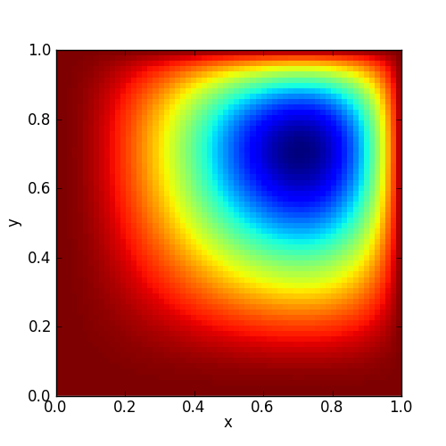
The mg_test_simple.py script solves a Poisson equation with a
known analytic solution. This particular example comes from the text
A Multigrid Tutorial, 2nd Ed., by Briggs. The example is:
on \([0,1] \times [0,1]\) with \(u = 0\) on the boundary.
The solution to this is shown below.
Since this has a known analytic solution:
We can assess the convergence of our solver by running at a variety of resolutions and computing the norm of the error with respect to the analytic solution. This is shown below:
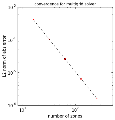
The dotted line is 2nd order convergence, which we match perfectly.
The movie below shows the smoothing at each level to realize this solution:
You can run this example locally by running the mg_vis.py script:
./examples/multigrid/mg_vis.py
projection
Another example uses multigrid to extract the divergence free part of a velocity field. This is run as:
./examples/multigrid/project_periodic.py
Given a vector field, \(U\), we can decompose it into a divergence free part, \(U_d\), and the gradient of a scalar, \(\phi\):
We can project out the divergence free part by taking the divergence, leading to an elliptic equation:
The project-periodic.py script starts with a divergence free
velocity field, adds to it the gradient of a scalar, and then projects
it to recover the divergence free part. The error can found by
comparing the original velocity field to the recovered field. The
results are shown below:
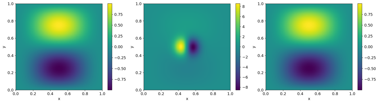
Left is the original u velocity, middle is the modified field after adding the gradient of the scalar, and right is the recovered field.
Exercises
Explorations
- Try doing just smoothing, no multigrid. Show that it still converges second order if you use enough iterations, but that the amount of time needed to get a solution is much greater.
Extensions
- Implement inhomogeneous dirichlet boundary conditions
- Add a different bottom solver to the multigrid algorithm
- Make the multigrid solver work for non-square domains