Compressible hydrodynamics solvers

The Euler equations of compressible hydrodynamics take the form:

\[\begin{split}\frac{\partial \rho}{\partial t} + \nabla \cdot (\rho U) &= 0 \\ \frac{\partial (\rho U)}{\partial t} + \nabla \cdot (\rho U U) + \nabla p &= \rho g \\ \frac{\partial (\rho E)}{\partial t} + \nabla \cdot [(\rho E + p ) U] &= \rho U \cdot g\end{split}\]

with \(\rho E = \rho e + \frac{1}{2} \rho |U|^2\) and \(p = p(\rho, e)\). Note these do not include any dissipation terms, since they are usually negligible in astrophysics.

pyro has several compressible solvers to solve this equation set. The implementations here have flattening at shocks, artificial viscosity, a simple gamma-law equation of state, and (in some cases) a choice of Riemann solvers. Optional constant gravity in the vertical direction is allowed.

Note

All the compressible solvers share the same problems/ directory, which lives in compressible/problems/. For the other compressible solvers, we simply use a symbolic-link to this directory in the solver’s directory.

compressible solver

compressible is based on a directionally unsplit (the corner transport upwind algorithm) piecewise linear method for the Euler equations, following [Colella90]. This is overall second-order accurate.

The parameters for this solver are:

• section: [compressible]

  option	value	description
  use_flattening	1	apply flattening at shocks (1)
  z0	0.75	flattening z0 parameter
  z1	0.85	flattening z1 parameter
  delta	0.33	flattening delta parameter
  cvisc	0.1	artifical viscosity coefficient
  limiter	2	limiter (0 = none, 1 = 2nd order, 2 = 4th order)
  grav	0.0	gravitational acceleration (in y-direction)
  riemann	HLLC	HLLC or CGF

• section: [driver]

  option	value	description
  cfl	0.8

• section: [eos]

  option	value	description
  gamma	1.4	pres = rho ener (gamma - 1)

• section: [particles]

  option	value	description
  do_particles	0
  particle_generator	grid

compressible_rk solver

compressible_rk uses a method of lines time-integration approach with piecewise linear spatial reconstruction for the Euler equations. This is overall second-order accurate.

The parameters for this solver are:

• section: [compressible]

  option	value	description
  use_flattening	1	apply flattening at shocks (1)
  z0	0.75	flattening z0 parameter
  z1	0.85	flattening z1 parameter
  delta	0.33	flattening delta parameter
  cvisc	0.1	artifical viscosity coefficient
  limiter	2	limiter (0 = none, 1 = 2nd order, 2 = 4th order)
  temporal_method	RK4	integration method (see mesh/integration.py)
  grav	0.0	gravitational acceleration (in y-direction)
  riemann	HLLC	HLLC or CGF
  well_balanced	0	use a well-balanced scheme to keep the model in hydrostatic equilibrium

• section: [driver]

  option	value	description
  cfl	0.8

• section: [eos]

  option	value	description
  gamma	1.4	pres = rho ener (gamma - 1)

compressible_fv4 solver

compressible_fv4 uses a 4th order accurate method with RK4 time integration, following [McCorquodaleColella11].

The parameter for this solver are:

• section: [compressible]

  option	value	description
  use_flattening	1	apply flattening at shocks (1)
  z0	0.75	flattening z0 parameter
  z1	0.85	flattening z1 parameter
  delta	0.33	flattening delta parameter
  cvisc	0.1	artifical viscosity coefficient
  limiter	2	limiter (0 = none, 1 = 2nd order, 2 = 4th order)
  temporal_method	RK4	integration method (see mesh/integration.py)
  grav	0.0	gravitational acceleration (in y-direction)

• section: [driver]

  option	value	description
  cfl	0.8

• section: [eos]

  option	value	description
  gamma	1.4	pres = rho ener (gamma - 1)

compressible_sdc solver

compressible_sdc uses a 4th order accurate method with spectral-deferred correction (SDC) for the time integration. This shares much in common with the compressible_fv4 solver, aside from how the time-integration is handled.

The parameters for this solver are:

• section: [compressible]

  option	value	description
  use_flattening	1	apply flattening at shocks (1)
  z0	0.75	flattening z0 parameter
  z1	0.85	flattening z1 parameter
  delta	0.33	flattening delta parameter
  cvisc	0.1	artifical viscosity coefficient
  limiter	2	limiter (0 = none, 1 = 2nd order, 2 = 4th order)
  temporal_method	RK4	integration method (see mesh/integration.py)
  grav	0.0	gravitational acceleration (in y-direction)

• section: [driver]

  option	value	description
  cfl	0.8

• section: [eos]

  option	value	description
  gamma	1.4	pres = rho ener (gamma - 1)

Example problems

Note

The 4th-order accurate solver (compressible_fv4) requires that the initialization create cell-averages accurate to 4th-order. To allow for all the solvers to use the same problem setups, we assume that the initialization routines initialize cell-centers (which is fine for 2nd-order accuracy), and the preevolve() method will convert these to cell-averages automatically after initialization.

Sod

The Sod problem is a standard hydrodynamics problem. It is a one-dimensional shock tube (two states separated by an interface), that exhibits all three hydrodynamic waves: a shock, contact, and rarefaction. Furthermore, there are exact solutions for a gamma-law equation of state, so we can check our solution against these exact solutions. See Toro’s book for details on this problem and the exact Riemann solver.

Because it is one-dimensional, we run it in narrow domains in the x- or y-directions. It can be run as:

./pyro.py compressible sod inputs.sod.x
./pyro.py compressible sod inputs.sod.y

A simple script, sod_compare.py in analysis/ will read a pyro output file and plot the solution over the exact Sod solution. Below we see the result for a Sod run with 128 points in the x-direction, gamma = 1.4, and run until t = 0.2 s.

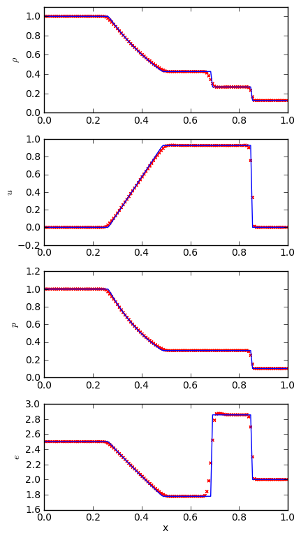
We see excellent agreement for all quantities. The shock wave is very steep, as expected. The contact wave is smeared out over ~5 zones—this is discussed in the notes above, and can be improved in the PPM method with contact steepening.

Sedov

The Sedov blast wave problem is another standard test with an analytic solution (Sedov 1959). A lot of energy is point into a point in a uniform medium and a blast wave propagates outward. The Sedov problem is run as:

./pyro.py compressible sedov inputs.sedov

The video below shows the output from a 128 x 128 grid with the energy put in a radius of 0.0125 surrounding the center of the domain. A gamma-law EOS with gamma = 1.4 is used, and we run until 0.1

We see some grid effects because it is hard to initialize a small circular explosion on a rectangular grid. To compare to the analytic solution, we need to radially bin the data. Since this is a 2-d explosion, the physical geometry it represents is a cylindrical blast wave, so we compare to Sedov’s cylindrical solution. The radial binning is done with the sedov_compare.py script in analysis/

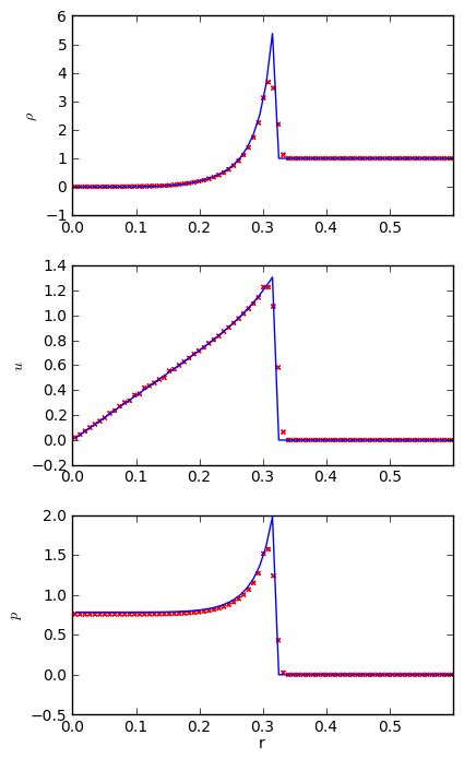
This shows good agreement with the analytic solution.

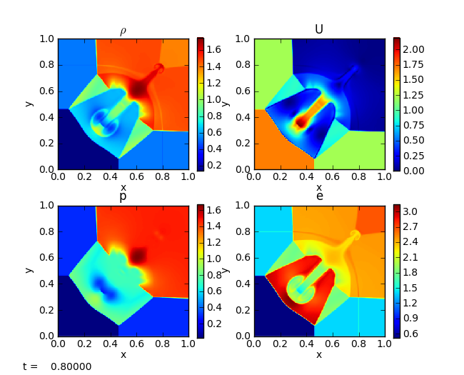
quad

The quad problem sets up different states in four regions of the domain and watches the complex interfaces that develop as shocks interact. This problem has appeared in several places (and a detailed investigation is online by Pawel Artymowicz). It is run as:

./pyro.py compressible quad inputs.quad

rt

The Rayleigh-Taylor problem puts a dense fluid over a lighter one and perturbs the interface with a sinusoidal velocity. Hydrostatic boundary conditions are used to ensure any initial pressure waves can escape the domain. It is run as:

./pyro.py compressible rt inputs.rt

bubble

The bubble problem initializes a hot spot in a stratified domain and watches it buoyantly rise and roll up. This is run as:

./pyro.py compressible bubble inputs.bubble

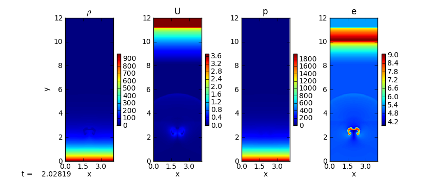
The shock at the top of the domain is because we cut off the stratified atmosphere at some low density and the resulting material above that rains down on our atmosphere. Also note the acoustic signal propagating outward from the bubble (visible in the U and e panels).

Exercises

Explorations

• Measure the growth rate of the Rayleigh-Taylor instability for different wavenumbers.

• There are multiple Riemann solvers in the compressible algorithm. Run the same problem with the different Riemann solvers and look at the differences. Toro’s text is a good book to help understand what is happening.

• Run the problems with and without limiting—do you notice any overshoots?

Extensions

• Limit on the characteristic variables instead of the primitive variables. What changes do you see? (the notes show how to implement this change.)

• Add passively advected species to the solver.

• Add an external heating term to the equations.

• Add 2-d axisymmetric coordinates (r-z) to the solver. This is discussed in the notes. Run the Sedov problem with the explosion on the symmetric axis—now the solution will behave like the spherical sedov explosion instead of the cylindrical explosion.

• Swap the piecewise linear reconstruction for piecewise parabolic (PPM). The notes and the Miller and Colella paper provide a good basis for this. Research the Roe Riemann solver and implement it in pyro.

Going further

The compressible algorithm presented here is essentially the single-grid hydrodynamics algorithm used in the Castro code—an adaptive mesh radiation hydrodynamics code developed at CCSE/LBNL. Castro is freely available for download.

A simple, pure Fortran, 1-d compressible hydrodynamics code that does piecewise constant, linear, or parabolic (PPM) reconstruction is also available. See the hydro1d page.